Visualising Financial Data In a Google Spreadsheet Motion Chart

Following on from Data Scraping Wikipedia With Google Spreadsheets, here’s a quick post showing how you can use another handy Google spreadsheet formula:

=GoogleFinance(“symbol”, “attribute”, “start_date”, “end_date”, “interval”)

This function will pull in live – and historical – price data for a stock.

Although I noticed this formula yesterday as I was exploring the “importHTML” formula described in the Wikipedia crawling post, I didn’t have time to have a play with it; but after a quick crib of HOWTO – track stocks in Google Spreadsheets, it struck me that here was something I could have fun with in a motion chart (you know, one of those Hans Rosling Gapminder charts….;-)

NB For the “official” documentation, try here: Google Docs Help – Functions: GoogleFinance)

# Stock quotes and other data may be delayed up to 20 minutes. Information is provided “as is” and solely for informational purposes, not for trading purposes or advice. For more information, please read our Stock Quotes Disclaimer.
# You can enter 250 GoogleFinance functions in a single spreadsheet; two functions in the same cell count as two.

So – let’s have some fun…

Fire up a new Google spreadsheet from http://docs.google.com, give the spreadsheet a name, and save it, and then create a new sheet within the spreadsheet (click on the “Add new sheet” button at the bottom of the page). Select the new sheet (called “Sheet2” probably), and in cell A1 add the following:

=GoogleFinance(“AAPL”, “all”, “1/1/2008”, “10/10/2008”, “WEEKLY”)

In case you didn’t know, AAPL is the stock ticker for Apple. (You can find stock ticker symbols for other companies on many finance sites.)

The formula will pull in the historical price data for Apple at weekly intervals from the start of 2008 to October 10th. (“all” in the formula means that all historical data will be pulled in on each sample date: opening price, closing price, high and low price, and volume.)

(If this was the live – rather than historical – data, it would be updated regularly, automatically…)

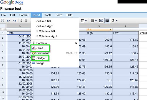
It’s easy to plot this data using a Google chart or a Google gadget:

I’m not sure a bar chart or scatter chart are quite right for historical stock pricing… so how about a line chart:

Et voila:

If you want to embed this image, you can:

If I was using live pricing data, I think the image would update with the data…?

Now create a few more sheets in your spreadsheet, and into cell A1 of this new sheet (sheet3) paste the following:

=GoogleFinance(“IBM”, “all”, “1/1/2008”, “10/10/2008”, “WEEKLY”)

This will pull in the historical price data for IBM.

Create two or three more new sheets, and in cell A1 of each pull in some more stock data (e.g. MSFT for Microsoft, YHOO for Yahoo, and GOOG…)

Now click on Sheet1, which should be empty. Fill in the following title cells by hand across cells A1 to G1:

Now for some magic…

Look at the URL of your spreadsheet in the browser address bar – mine’s “http://spreadsheets.google.com/ccc?key=p1rHUqg4g423seyxs3O31LA&hl=en_GB#”

That key value – the value between “key=” and “&hl=en_GB#” is important – to all intents and purposes it’s the name of the spreadsheet. Generally, the key will be the characters between “key=” and an “&” or the end of the URL; the “&” means “and here’s another variable” – it’s not part of the key.

In cell B2, enter the following:

=ImportRange(“YOURKEY”, “Sheet2!A2:F42”)

YOURKEY is, err, your spreadsheet key… So here’s mine:

=ImportRange(“p1rHUqg4g423seyxs3O31LA”, “Sheet2!A2:F42”)

What ImportRange does is pull in a range of cell values from another spreadsheet. In this case, I’m pulling in the AAPL historical price data from Sheet2 (but using a different spreadsheet key, I could pull in data from a different spreadsheet altogether, if I’ve made that spreadsheet public).

In cell A2, enter the ticker symbol AAPL; highlight cell A2, click on the square in the bottom right hand corner and drag it down the column – when you release the mouse, the AAPL stock ticker should be added to all the cells above. Label each row from the imported data, and then in the next row, B column, import the data from Sheet 3:

These rows will need labeling “IBM”.

Import some more data if you like and then… let’s create a motion chart (info about motion charts.

Highlight all the cells in sheet1 (all the imported data from the other sheets) and then from the Insert menu select Gadget; from the Gadget panel that pops up, we want a motion chart:

Configure the chart, and have a play [DEMO]:

Enjoy (hit the play button… :-)

PS And remember, you could always export the data from the spreadsheet – though there are probably better API powered ways of getting hold of that data…

PPS and before the post-hegemonic backlash begins (the .org link is broken btw? or is that the point?;-) this post isn’t intended to show how to use the Google formula or the Motion Chart well or even appropriately, it’s just to show how to use it to get something done in a hacky mashery way, with no heed to best practice… the post should be viewed as a quick corridor conversation that demonstrates the tech in a casual way, at the end of a long day…

PS for a version of this post in French, see here: Créer un graphique de mouvement à partir de Google Docs.